Colbyn's School Notes
Meta
Miscellaneous
Functional Utilities & Notation Conveniences
Right to Left Evaluation
Left to Right Evaluation
Derivative Shorthand
For this notation, the derivative with respect to a given variable, is implicit.
Radians & Radian Conversion
Constants
Conversion
Constants
ℯ (Euler's number)
Algebra
Properties
Trigonometry
Trigonometric Identities
Pythagorean Identities
Sum and Difference Identities
Cofunction Identities
Ratio Identities
Double-Angle Identities
Half-Angle Identities
Power-Reducing Identities
Product-to-Sum Identities
Sum-to-Product-Identities
Trigonometric Equations
Euler's Formula
Coordinate & Number Systems
Polar Coordinate System
Given
Then
Properties
Given
Then
De Moivre’s Theorem
De Moivre’s Theorem For Finding Roots
Trigonometric form of a complex number
Vectors
Quick Facts
-
Two vectors are equal if they share the same magnitude and direction.
Initial points don't matter. -
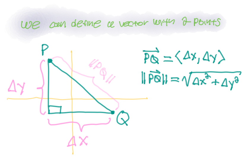
You can define a vector with two points.
-
Do not divide vectors!
- \(\vec{v} \cdot \vec{v} = ||\vec{v}||^2 \implies \text{constant}\)
- \(\vec{v} \cdot \left(\vec{v}\right)^\prime = 0\)
Vector Operations
Dot Product
Cross Product
Length of a Vector
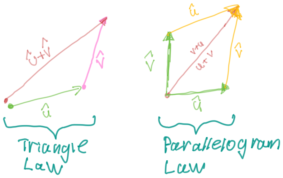
Definition of Vector Addition
If \(\vec{u}\) and \(\vec{v}\) are positioned so the initial point of \(\vec{v}\) is at the terminal point of \(\vec{u}\), then the sum \(\vec{u} + \vec{v}\) is the vector from the initial point of \(\vec{u}\) to the terminal point of \(\vec{v}\).
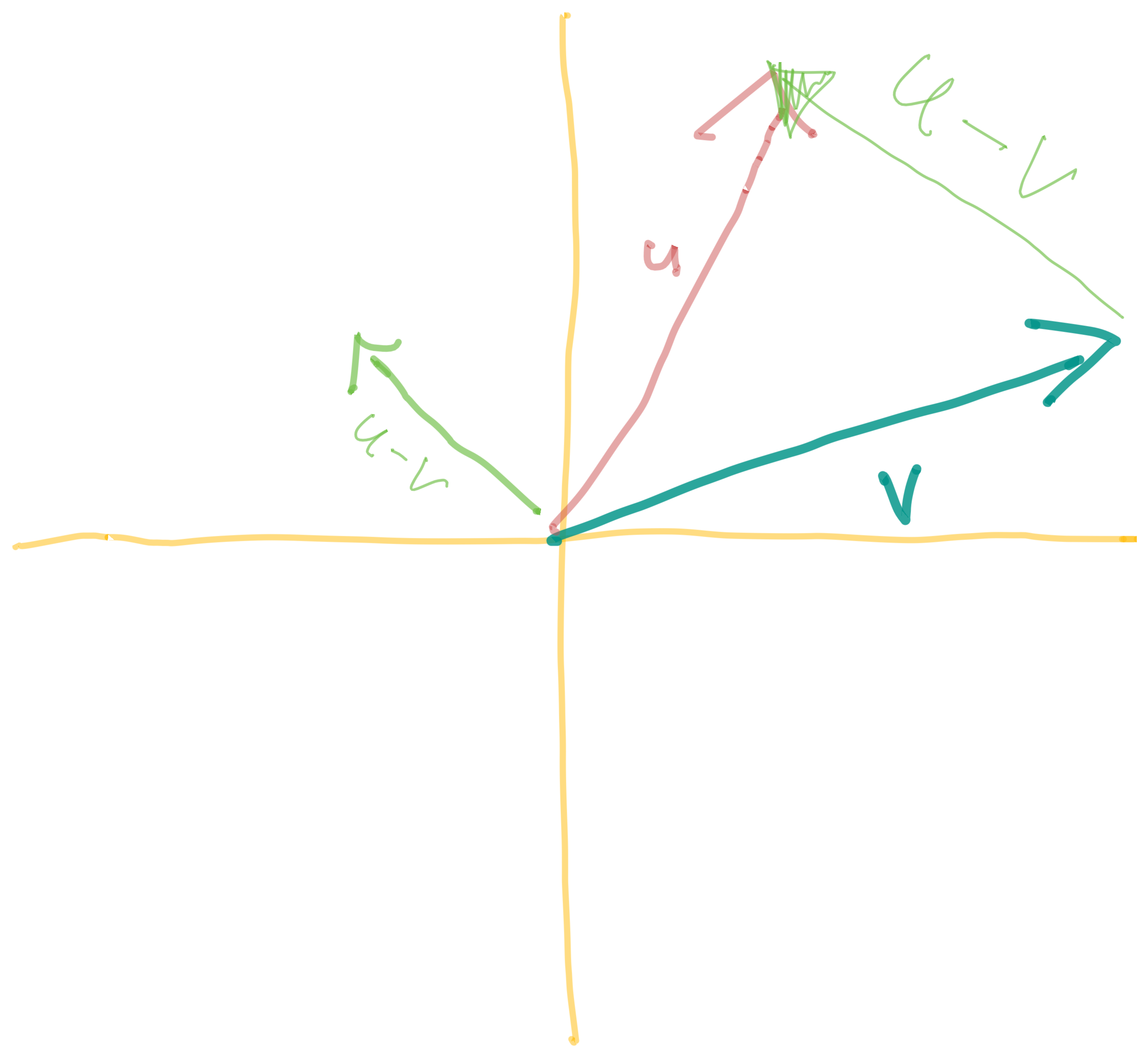
Given some vectors \(\vec{u}\) and \(\vec{v}\), the vector \(\vec{u} - \vec{v}\) is the vector that points from the head of \(\vec{v}\) to the head of \(\vec{u}\)
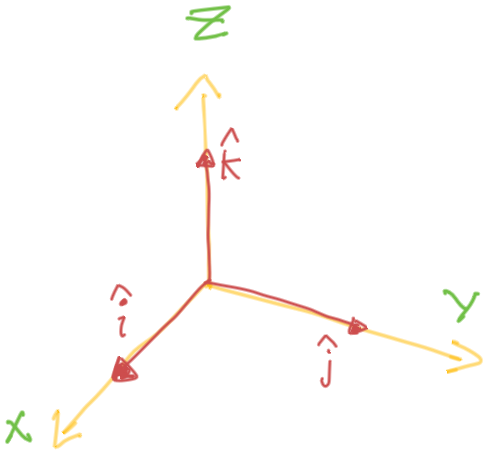
Standard Basis Vectors
Orthogonal
Two vectors are orthogonal if and only if
The Unit Vector
If \(\theta\) is the angle between the vectors \(\vec{a}\) and \(\vec{b}\), then
If \(\theta\) is the angle between the nonzero vectors \(\vec{a}\) and \(\vec{b}\), then
Two nonzero vectors \(\vec{a}\) and \(\vec{b}\) are parallel if and only if
Properties of the Dot Product
Direction Cosines & Direction Angles of a Vector
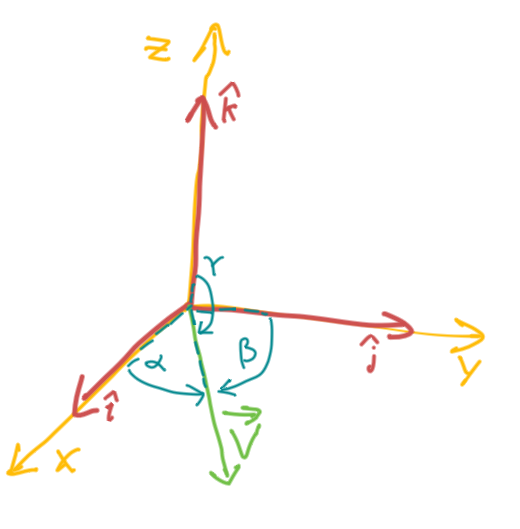
Where
Direction Cosines
Direction Angles
Theorem
Proof
Given
Therefore
Vector Relations
Parallel Vectors
- When two vectors are parallel; they never intersect (duh).
Given some vectors
The vectors \(\vec{a}\) and \(\vec{b}\) are parallel if and only if they are scalar multiples of one another.
Alternatively
Orthogonal Vectors
- When two vectors are orthogonal; they meet at right angles.
Given some vectors
Two vectors are orthogonal if and only if
Reparameterization of the position vector \(\vec{v}(t)\) in terms of length \(S(t)\)
-
We can parametrize a curve with respect to arc length; because arc length arises naturally from the shape of the curve and does not depend on any coordinate system.
The Arc Length Function
Given
We can redefine \(\vec{v}\) in terms of arc length between two endpoints
That is, \(S(t)\) is the length of the curve (\(C\)) between \(r(a)\) and \(r(b)\).
Furthermore from the adjacent definition; we can simply the above to
The Arc Length Function
That is
Vectors Derived From Some Curve Defined by \(\vec{v}\)
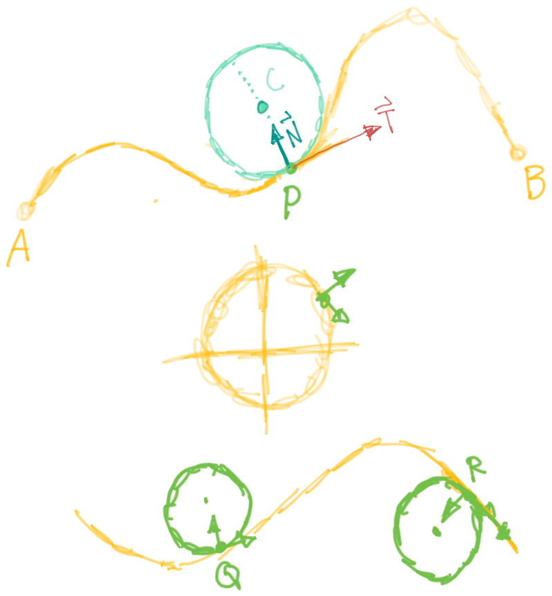
The Unit Vector
The Unit Tangent Vector
The Unit Normal Vector
The Binormal Vector
-
Therefore, the binormal vector is orthogonal to both the tangent vector and the normal vector.
-
The plane determined by the normal and binormal vectors N and B at a point P on a curve C is called the normal plane of C at P.
-
The plane determined by the vectors T and N is called the osculating plane of C at P. The name comes from the Latin osculum, meaning “kiss.” It is the plane that comes closest to containing the part of the curve near P. (For a plane curve, the osculating plane is simply the plane that contains the curve.)
Kappa - Curvature of a Vector
Tangential & Normal Components of the Acceleration Vector of the Curve
When we study the motion of a particle, it is often useful to resolve the acceleration into two components, one in the direction of the tangent and the other in the direction of the normal.
Specifically
Vector Calculus
The Position Vector \(\vec{r}(t)\)
(Original Function)
The Velocity Vector \(\vec{v}(t)\)
(First Derivative)
- The velocity vector is also the tangent vector and points in the direction of the tangent line.
- The speed of the particle at time t is the magnitude of the velocity vector, that is,
$$\begin{equation} \begin{split} \underbrace{|\vec{v}(t)| = |(\vec{r})^\prime(t)| = \frac{\mathrm{d}s}{\mathrm{d}t}} _{\text{rate of change of distance with respect to time}} \end{split} \end{equation}$$
The Acceleration Vector \(\vec{a}(t)\)
(Second Derivative)
Matrices
Reference
The Determinant of A Matrix
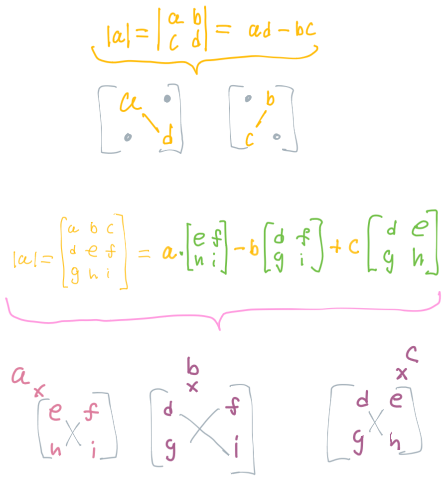
Only works for square matrices.
The Cross Product
Geometry
Definition of a Line
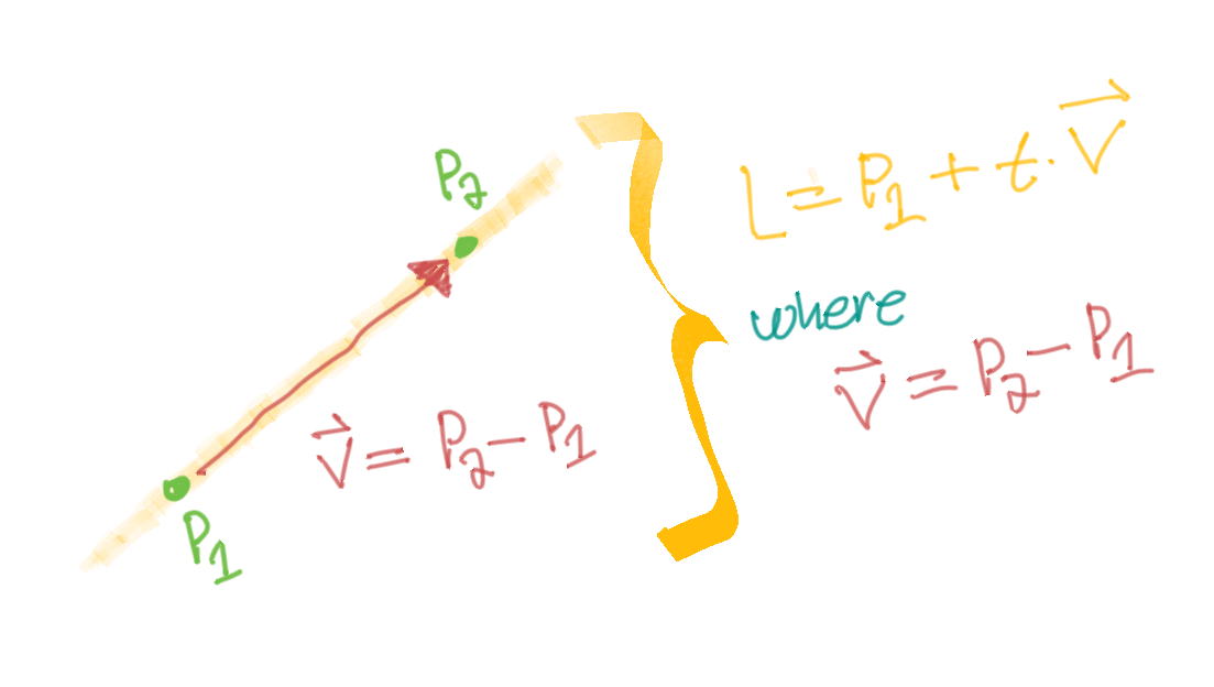
Vector Equation of a Line
Given
We can define a vector between \(\colorB{P_1}\) and \(\colorC{P_2}\)
Therefore
The equation of a line in 3D space or \(\mathbb{R}^3\) can be defined VIA the following options
That is
Parametric Equation of a Line
Essentially
That is, \(t\) is the scaling factor. In a way, it's like it's a function of \(t\), but also similar to the slope (\(m\)) in \(y = mx + b\), except \(m\) (i.e. \(t\)) is parameterized.
Sometimes this will be (confusingly) denoted as
Symmetric Equation of a Line
Therefore
Rationale
We rewrite \(r = r_0 + a = r_0 + t v\) in terms of \(t\).
That is
Parameterizations of a curve
- Parametrized curve
- A curve in the plane is said to be parameterized if the set of coordinates on the curve, (x,y), are represented as functions of a variable t.
- A parametrized Curve is a path in the xy-plane traced out by the point \(\left(x(t), y(t)\right)\) as the parameter \(t\) ranges over an interval \(I\).
- A parametrized Curve is a path in the xyz-plane traced out by the point \(\left(x(t), y(t), z(t)\right)\) as the parameter \(t\) ranges over an interval \(I\).
Curvature Properties
Length of a Curve
The Arc Length Function
Suppose
-
Given some curve \(C\) defined by some vector \(\vec{r}\) in \(\mathbb{R}^3\)
-
where \(r^\prime\) is continuous and \(C\) is traversed exactly once as \(t\) increases from \(a\) to \(b\)
We can define it's arc length function VIA
Limits
L’Hospital’s Rule
In other words, if L’Hospital’s Rule applies to indeterminate forms.
Limit Laws
Limit Formulas
Growth Rates
- Factorial functions grow faster than exponential functions.
- Exponential functions grow faster than polynomials.
Calculus
Derivative Tables
Integration Tables
Riemann Sums
Given
Left Riemann Sum
Right Riemann Sum
Midpoint Riemann Sum
We can also do away with the index notation and simplify things.
Trapezoidal Riemann Sum
Simpson's Rule
Improper Integrals
Infinite Sequences
Infinite Sequence
Helpful Theorem
Example
Example
Infinite Series
Infinite Series
Note that the limit of every convergent series is equal to zero. But the inverse isn't always true. If the limit is equal to zero, it may not be convergent.
For example, \(\sum_{n=1}^\infty \frac{1}{n}\) does diverge; but it's limit is equal to zero.
If the limit is equal to zero; the test is inconclusive.
Geometric Series
The Integral Test
Constraints on \([1,n)\)
- Continuous
- Positive
- Decreasing (i.e. use derivative test)
P-Series -or- Harmonic Series
Note: the Harmonic series is the special case where \(p=1\)
Comparison Test
Limit Comparison Test
Warning
- If \(L > 0\), this only means that the limit comparison test can be used. You still need to determine if either\(A_n\) or \(B_b\) converges or diverges.
- Therefore, this does not apply to any arbitrary rational function.
Notes
- For many series, we find a suitable comparison, \(B_n\), by keeping only the highest powers in the numerator and denominator of \(A_n\).
Estimating Infinite Series
Differential Equations
Separable Differential Equations
Growth and Decay Models
The above states that all solutions for \(y^\prime = k y\) are of the form \(y = C e^{k t}\).
Where
Exponential growth occurs when \(\textcolor{Periwinkle}{k > 0}\), and exponential decay occurs when \(\textcolor{Periwinkle}{k < 0}\).
The Law of Natural Growth:
The Logistic Model of Population Growth:
Where
Solving the Logistic Equation
Via partial fraction decomposition
Rewriting the differential equation
Second Order Homogeneous Linear Differential Equations with Constant Coefficients
Properties
-
If \(f(x)\) and \(g(x)\) are solutions; then \(f + g\) is also a solution. Therefore, the most general solution to some second order homogeneous linear differential equations with constant coefficients would be \(y = C_1 f(x) + C_2 g(x)\).
This is why, when you find two solutions to the characteristic equation \(r_1\) and \(r_2\) respectively, we write it like so.
\(r_1 = r_2\)
Given some:
We can presume that \(y\) is of the form \(e^{r t}\), and therefore:
Substituting this back into the original equation, we have:
Where:
So therefore:
Where the general solution is of the form:
Parametric Equations
First Derivative Formula
To find the derivative of a given function defined parametrically by the equations \(x = u(t)\) and \(y = v(t)\).
Second Derivative Formula
To find the second derivative of a given function defined parametrically by the equations \(x = u(t)\) and \(y = v(t)\).
The above shows different ways of representing \(\frac{\mathrm{d}^{2}y}{\mathrm{d}x^2}\). (I.e. it doesn't correspond to some final solution.)
Arc Length
Formula for the arc length of a parametric curve over the interval \([a, b]\).